So there I was, sitting in a car on the Autobahn as a passenger, laptop-less, armed with nothing but an Android phone and too much curiosity. The car had just been fitted with aftermarket BLE tire pressure sensors intended for Tesla vehicles. I wanted to know what they were saying.
This is the story of how I went from raw hex bytes to a live dashboard showing real-time tire pressure and temperature for all four wheels, entirely reverse engineered, with no documentation and no SDK.
The Hardware
The sensors are tsTPMS units, BLE tire pressure monitors that advertise themselves with Manufacturer ID 0x022B, which belongs to Tesla Motors. These are aftermarket sensors that use Tesla’s assigned Bluetooth company identifier. They are widely sold and are used in many non-Tesla vehicles as well.
Each sensor sits inside the wheel, rotating with it at highway speed and sending BLE notifications roughly every 20 seconds.
Step 1: Finding the Sensors
My first attempt was Termux on Android with Python plus bleak. That failed immediately:
FileNotFoundError: [Errno 2] No such file or directory
bleak expects a BLE stack that Termux does not provide in the same way as a normal desktop Linux setup, so I switched to LightBlue on the phone for the first reconnaissance pass.
LightBlue showed the sensors immediately:
| Field | Value |
|---|---|
| Name | tsTPMS |
| Manufacturer | Tesla Motors (0x022B) |
| Advertised service UUID | 00001122-0000-1000-8000-00805f9b34fb |
That advertised UUID is just what the sensor broadcasts to be discoverable. Once connected, a different custom GATT service appears with the actual data stream:
- Service UUID:
00000211-b2d1-43f0-9b88-960cebf8b91e - Characteristic “From Tire”:
00000213-b2d1-43f0-9b88-960cebf8b91e - Properties: Notify only
Once that was clear, I moved to Windows plus Python, where bleak worked fine for real logging and decoding.
pip install bleak matplotlib pandas numpy
Finding all four sensors by filtering for Manufacturer ID 555 (0x022B):
import asyncio
from bleak import BleakScanner

async def scan():
    devices = await BleakScanner.discover(timeout=20, return_adv=True)
    for address, (device, adv) in devices.items():
        if 555 in adv.manufacturer_data:
            print(f"TPMS: {device.name} | {address}")

asyncio.run(scan())
All four showed up:
TPMS: tsTPMS | D0:39:C9:37:0A:63
TPMS: tsTPMS | D0:39:86:1F:0A:A3
TPMS: tsTPMS | D0:39:40:20:0A:F3
TPMS: tsTPMS | D0:39:AC:58:0A:83
Step 2: Staring at Hex Bytes on the Autobahn
The normal sensor packet looked like this:
1208 e201 0508 cc02 1030
No documentation. No SDK. Just bytes.
The first useful step was not decoding, but logging. I wrote a script that dumped raw packets with timestamps and let me add manual comments while driving.
15:17:51 | 1208e2010508cc021030 | 120kmh
15:18:12 | 1208e2010508cc021032 | 120kmh
15:19:31 | 1208e2010508cf021034 | 120kmh
15:22:31 | 1208e2010508cf021038 | 100kmh
15:23:31 | 1208e2010508cf021038 | stau, schleichender verkehr
15:28:31 | 1208e2010508cf02103a | 110kmh ca
That turned out to be the key. Once the logs had timestamps and driving context, patterns started to emerge very quickly.
Step 3: Cracking the Protocol
The structure
Byte:  [0]  [1]  [2]  [3]  [4]  [5]  [6]  [7]  [8]  [9]
       12   08   E2   01   05   08   CC   02   10   30
Within the normal 10-byte data packet, bytes 0, 1, 3, 4, 5, and 8 stayed constant in my captures. The fields that changed were byte 2, bytes 6 to 7, and byte 9.
Temperature, byte 9
This was the first field that became obvious. In the early logs, byte 9 moved through values like 48, 50, 52, 54, 56, and 58 while the car was driven and later slowed down.
15:17  Byte[9] = 48  ->  48/2 = 24°C
15:20  Byte[9] = 52  ->  52/2 = 26°C
15:28  Byte[9] = 58  ->  58/2 = 29°C
A later full-session capture showed the same behavior much more clearly. Sensor A, for example, went from 23.0 °C at the start of the session to 30.0 °C during sustained highway driving, then dropped slightly again.
Best-fit interpretation:
Byte[9] / 2.0 = °C
Pressure, bytes 6 and 7
The next field was pressure. Bytes 6 and 7 varied only slightly, which is exactly what you would expect from tire pressure during one drive.
CC 02  ->  Little-endian 16-bit: 0x02CC = 716
CF 02  ->  0x02CF = 719
D2 02  ->  0x02D2 = 722
Testing several scaling ideas produced one result that landed in a realistic range:
| Formula | Result for 716 | Plausible? |
|---|---|---|
| Direct as kPa | 7.16 bar | No |
| ÷ 10 as kPa | 0.716 bar | No |
| × 0.25 kPa | 1.79 bar | Maybe, but too low |
| ÷ 300 | 2.387 bar | Yes |
Best-fit interpretation:
((Byte[7] << 8) | Byte[6]) / 300.0 = bar
The later laptop session supported that decode strongly. Across the full four-sensor viewer session, average pressures clustered between 2.386 and 2.433 bar, with very tight per-sensor ranges and a small upward drift as temperature increased.
Step 4: Full Session Validation
Once the protocol was mostly decoded, I built a live monitor and captured a longer session with all four sensors connected in parallel.
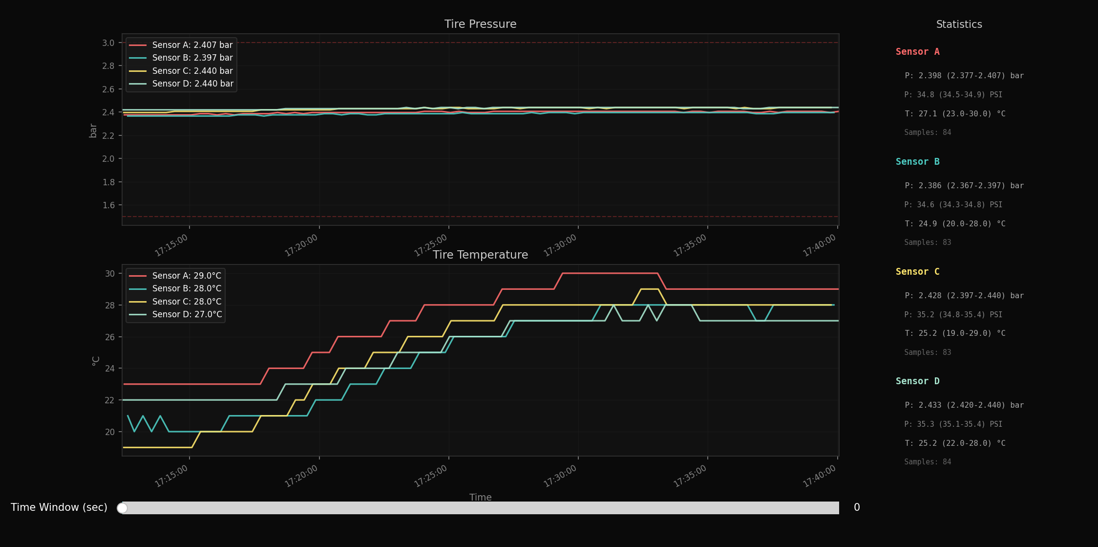
(Viewer output from the final Python monitor. Pressure is shown on top, temperature on the bottom, with per-sensor summary statistics on the right.)
Summary statistics from the viewer
| Sensor | Pressure avg (range) | PSI avg (range) | Temp avg (range) | Samples |
|---|---|---|---|---|
| Sensor A | 2.398 (2.377-2.407) bar | 34.8 (34.5-34.9) PSI | 27.1 (23.0-30.0) °C | 84 |
| Sensor B | 2.386 (2.367-2.397) bar | 34.6 (34.3-34.8) PSI | 24.9 (20.0-28.0) °C | 83 |
| Sensor C | 2.428 (2.397-2.440) bar | 35.2 (34.8-35.4) PSI | 25.2 (19.0-29.0) °C | 83 |
| Sensor D | 2.433 (2.420-2.440) bar | 35.3 (35.1-35.4) PSI | 25.2 (22.0-28.0) °C | 84 |
A few things stand out:
- The pressure values are very stable.
- The temperatures rise in discrete steps, which is exactly what you would expect from a raw byte divided by 2, meaning 0.5 °C resolution.
- Pressure rises slightly as the tires warm up, which is physically sensible.
- The sensors do not all follow the same thermal curve. At least two different thermal profiles are visible in the graph.
That is strong support for the pressure and temperature decode. It is not enough, by itself, to prove exact wheel positions. The graph suggests grouping behavior, but too many confounding factors remain, including recent driving history, sun exposure, parking orientation, and per-sensor offset.
Step 5: The Weird Packets
Not every packet was a normal pressure and temperature update. Two other packet families appeared in the logs.
The 19-byte packet, flag 0xEA
12 11 EA 01 0E 0A 04 32 68 EF 3E 12 03 1C 34 D7 18 A0 17
This appeared once per sensor connection, right after the first normal packet. It was identical across all four sensors in my captures.
That makes it unlikely to contain wheel-specific position data. My best guess is that it is some kind of session announcement, identification packet, or capability packet. The exact contents remain unknown.
The 0x92 packets
Two 0x92 variants appeared, one short and one extended.
10-byte variant
12 08 92 02 05 08 C0 25 10 19
13-byte variant
12 0B 92 02 08 08 80 96 01 10 64 18 01
These appeared roughly every four minutes and used values that were much larger than the normal pressure field. In the session report, the larger embedded value increased by about 9600 between intervals in one repeated pattern. That suggests some kind of cumulative counter, but I could not verify whether it represents distance, wheel rotations, calibration state, or something else. So for now, the safe conclusion is simple: these packets are real, periodic, and not part of the normal pressure and temperature payload.
Step 6: Which Wheel Is Which?
This is the part that is still open.
The viewer session clearly shows that the four sensors do not behave identically. There are pressure differences and thermal differences between them. But one driving session is not enough to assign exact physical positions with confidence.
What I can say:
- the sensors can be separated into plausible groups based on pressure and temperature behavior
- the graph shows different warm-up patterns
- a front/rear interpretation is possible
What I cannot say yet:
- which sensor is definitely front-left, front-right, rear-left, or rear-right
- whether the pressure split is vehicle-related or partly sensor calibration
- whether the earlier-heating sensors are truly the front axle in all cases
Two practical follow-up methods could resolve the wheel mapping more cleanly.
RSSI-based guessing: place the BLE receiver at a known position, for example near the front-left wheel or inside the driver’s footwell, and compare signal strength across the four sensors during repeated short scans. The closest sensor should, in principle, produce the strongest RSSI. This is useful as a quick heuristic, but not definitive, since BLE RSSI is noisy and can be affected by wheel orientation, bodywork, reflections, and multipath.
Spin-to-identify: jack up the car and spin one wheel at a time, then watch which sensor wakes up or updates first. That should provide a much stronger mapping signal than RSSI alone. A one-tire deflation test would work too.
Until then, any exact wheel mapping would be a hypothesis, not a result.
The Final Script
By the end of the session, I had a monitor that connected to all four sensors in parallel, auto-reconnected on disconnects, plotted live pressure and temperature, and wrote annotated CSV logs.
SENSORS = {
    "D0:39:C9:37:0A:63": "SENSOR_A",
    "D0:39:86:1F:0A:A3": "SENSOR_B",
    "D0:39:40:20:0A:F3": "SENSOR_C",
    "D0:39:AC:58:0A:83": "SENSOR_D",
}

def decode(raw):
    if len(raw) == 10 and raw[2] == 0xE2:
        pressure_bar = ((raw[7] << 8) | raw[6]) / 300.0
        temp_c = raw[9] / 2.0
        return pressure_bar, temp_c
I deliberately kept the labels neutral here. Until I do a one-tire test, neutral sensor IDs are more honest than pretending the wheel mapping is fully solved.
Protocol Summary
Normal data packet (10 bytes):
┌──────┬──────┬──────┬──────┬──────┬──────┬──────┬──────┬──────┬──────┐
│  B0  │  B1  │  B2  │  B3  │  B4  │  B5  │  B6  │  B7  │  B8  │  B9  │
│ 0x12 │ 0x08 │ 0xE2 │ 0x01 │ 0x05 │ 0x08 │ PrLo │ PrHi │ 0x10 │ Temp │
└──────┴──────┴──────┴──────┴──────┴──────┴──────┴──────┴──────┴──────┘

Pressure:    ((B7 << 8) | B6) / 300.0  ->  bar
Temperature: B9 / 2.0                   ->  °C

Observed packet types:
  B2 = 0xE2, 10 bytes       -> normal data, about every 20 seconds
  B2 = 0xEA, 19 bytes       -> connection-time announcement packet
  B2 = 0x92, 10 or 13 bytes -> periodic special packet, meaning still unknown

GATT Characteristic: 00000213-b2d1-43f0-9b88-960cebf8b91e
Service UUID:        00000211-b2d1-43f0-9b88-960cebf8b91e
Manufacturer ID:     0x022B (Tesla Motors)
What Is Still Open
Exact wheel mapping
I still cannot assign exact tire positions from this dataset alone.Meaning of the
0x92packets
They look like periodic bookkeeping or cumulative state, but they are not decoded yet.Meaning of the 19-byte
0xEApacket
It is probably a connection-time identification or capability packet, but that is still a hypothesis.Whether
/300is the exact vendor scaling
It matches the data very well, but I still treat it as an empirical decode.
Lessons Learned
This is the workflow that worked well for reverse engineering BLE sensors with no documentation:
- Use LightBlue first.
- Log everything raw before trying to decode anything.
- Add real-world annotations while collecting data.
- Validate one field at a time.
- Keep your conclusions narrower than your excitement.
The most important part was not clever math. It was having timestamps, raw payloads, and enough real-world context to test ideas against reality.
That is what turned random hex into a protocol.